Common Distance Metrics Implemented in Ruby

Introduction

The starting point for many machine learning tasks is to describe your entities in terms of a set of features. For example, in text-based learning your features might be the frequency of different words, or for an image-based task your starting features could be pixel intensity values. Typically we attempt to represent our entities as an array of numerical elements, amenable to machine learning algorithms.

When represented in this format it is often useful to consider which entities are 'close together'. This concept of proximity is important for clustering algorithms, nearest-neighbour algorithms, generating recommendations and much more. But how do we calculate the distance between two vectors?

There are several different ways to approach this and we introduce each of these measures, before showing how they can be impemented in ruby:

• Euclidean Distance
• Manhattan Distance
• Chebyshev Distance
• Minkowski Distance
• Hamming Distance
• Cosine Distance
• Jaccard Distance

Let's get started.

Euclidean Distance

This is the intuitive measure of distance which we derive from our 2D and 3D experiences of the world around us, but this measure can be generalized to any number of dimensions. If we have two vectors of dimension $N$, $\mathbf{a} = \left[ a_{1}, a_{2}, \ldots, a_{N} \right]$ and $\mathbf{b} = \left[ b_{1}, b_{2}, \ldots b_{N}\right]$, then we denote the Euclidean distance between them as $D_{\rm{euclidean}} \left( \mathbf{a}, \mathbf{b} \right)$ where:

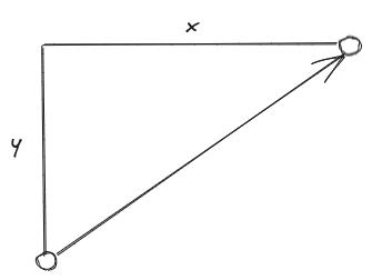
Taking the square root of the overall sum of squared differences in each dimension, this measure is really just an extension of Pythagorean theorem to $N$ dimensions:

    
  def self.euclidean_distance(a,b)
    return unless a.any? && (a.size == b.size)

    diff_squared = (0..a.size-1).reduce(0) do |sum, i|
      sum + (a[i] - b[i])**2
    end
    Math.sqrt(diff_squared)
  end
    
  

You can see this implementation (with specs), along with the other measures presented in this post, on GitHub.

We note the guard clause which ensures that both vectors are of the same length. In general, these distance metrics do not make much sense if we try to compare two vectors that occupy different dimensional spaces. In a similar way, we do not attempt to calculate the distance when passed an empty vector. You will see a similar guard clause in the implementation of most of these other measures. There will be slightly different conditions imposed on the Cosine similarity and Jaccard distance measures, which we will discuss later.

Manhattan Distance

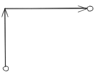
The Manhattan distance is, in some ways, a simpler metric than the Euclidean distance. It is also know as the City Block distance, because, in two-dimensions, the path taken between the two points can be likened to the path you would take to navigate around the blocks of city street grid-system,. Instead of taking the shortest path between the two points, we are restricted to travel along the direction of the axes of our grid system, e.g.

The Manhattan distance between our $N$-dimensional vectors, $\mathbf{a}$ and $\mathbf{b}$, is denoted $ D_{\rm{manhattan}} \left( \mathbf{a}, \mathbf{b} \right)$ and can be calculated as follows:

The metric can be calculated in ruby as follows:

    
  def self.manhattan_distance(a, b)
    return unless a.any? && (a.size == b.size)

    (0..a.size-1).reduce(0) do |sum, i|
      sum + (a[i] - b[i]).abs
    end
  end
    
  

Chebyshev Distance

Chebyshev distance considers the separation in only a single dimension, that for which the point separation is greatest. Try to imagine that we collapse all the other coordinates unto a single axis, and then consider the separation of the points on that axis.

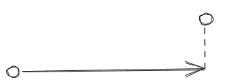
Using the same vector notations as already established, the Chebyshev distance, denoted as $D_{chebyshev}$, is calculated as

An implementation of this metric in ruby is show below:

    
  def self.chebyshev_distance(a, b)
    return unless a.any? && (a.size == b.size)

    (0..a.size-1).map do |i|
      (a[i] - b[i]).abs
    end.max
  end
    
  

Minkowski Distance

The Minkowski distance can be considered as a generalization of the three measures that we have already introduced. It introduces a new parameter, $p$, such that the separation in each dimension is raised to the power of $p$. We then sum these terms over all $N$ dimensions before taking the $p^{\rm{th}}$ root. I.e.

We can implement this measure in ruby as follows:

    
  def self.minkowski_distance(a, b, p)
    return unless a.any? && (a.size == b.size)

    (0..a.size-1).reduce(0) do |sum, i|
      sum + (a[i] - b[i]).abs**p
    end**(1.0/p)
  end
    
  

The Minkowski distance is identical to the Manhattan distance when $p=1$ and is identical to the Euclidean distance when $p=2$.

The equivalence to $D_{\rm{chebyshev}}$ in the limit of $p \to \infty$ is not just as obvious, but you hopefully you can appreciate that as the exponent $p$ gets larger, then the term $\sum_{i=1}^{N} \left| a_{i} - b_{i} \right|^{p \to \infty}$ will be dominated by the single dimension with the biggest difference, with the other dimensions contributing less and less. We can exercise this limit in our specs for the method as follows:

    
    describe "when p = 1_000" do
      let(:p) { 1_000 }
      let(:examples) do
        [
          [[0, 1, 2], [1, 2, 0]],
          [[0,0], [1,0]],
          [[-1,0], [1,0]],
          [[0,0,0,0], [1,0,1,0]],
        ]
      end

      it "should approach the chebyshev distance" do
        examples.each do |vectors|
          expect(Metrics.minkowski_distance(vectors[0], vectors[1], p))
            .to be_within(0.001).of Metrics.chebyshev_distance(vectors[0], vectors[1])
        end
      end
    end
  end
    
  

Hamming Distance

The Hamming distance compares two vectors element-by-element and increments the distance by 1 for each index where the elements differ. It is frequently encountered when comparing strings of characters or digits. Because this measure is only concerned about comparing the identity of elements at each index in our two arrays, it can be applied in either a numerical or non-numberical context; a flexibility which we do not have with the other measures, such as $D_{\rm{euclidean}}$.

For example, we can consider the Hamming distance between two words to measure how different they are. For example we compare the words 'happy' and 'hippo' in the image below:

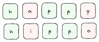
This distance measure is probably easier understood with the depiction above, but in the interest of maintaining some sort of mathematical rigor we can represent $D_{\rm{hamming}}$ as follows:

$$ \begin{aligned} D_{\rm{hamming}} \left( \mathbf{a}, \mathbf{b} \right) = \sum_{i=1}^{N} d_{i} \tag{5}\label{5} \end{aligned} $$ where \[ d_{i} = \left\{ \begin{array}{ll} 1 & a_{i} \neq b_{i}\\ 0 & \rm{otherwise} \\ \end{array} \right. \]

We can calculate this metric in ruby as follows:

    
  def self.hamming_distance(a, b)
    return unless a.any? && (a.size == b.size)

    (0..a.size-1).reduce(0) do |sum, i|
      sum + ((a[i] != b[i]) ? 1 : 0)
    end
  end
    
  

Cosine Distance

The Cosine similarity describes if two vectors are pointing in a similar direction. The measure ranges from -1 though to +1.

If the vectors are pointing in the same direction then $\cos(\theta) = \cos(0) = 1$, but if the vectors are orthoganal to one another (i.e. at right angles) then $\cos(\theta) = \cos(90\degree) = 0$. If the vectors are pointing in exactly opposing directions then $\cos(\theta) = \cos(180\degree) = -1$.

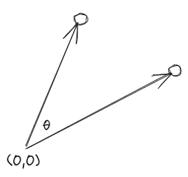
Note that this metric is independent of the size of the vectors involved, it is solely their direction which is important. This feature can be very useful in some circumstances and negates the need to carry out normalization of your vectors. For example, if we consider the case of text similarity and suppose we represent our differnt text samples using a bag-of-words model. In this model each index in the array represents a word in our vocabulary/dictionary, and the value at that index is the number of times the word has occured in the text sample. In this way each text sample is represented by a large (potentially sparse) array of frequencies. Some text samples could be very long and some could be very short, but these can still be meaningfully compared using cosine similarity, as it is only the relative frequency of the different words which is important.

We can use our established vector notation for this measure also, but in this case we are talking about a similarity rather than a distance so we shall denote the quantity as $S_{\rm{cosine}}$. It is calculated as follows:

Here the numerator, $\mathbf{a} \cdot \mathbf{b}$, represents the dot-product of the vectors $\mathbf{a}$ and $\mathbf{b}$, whilst $\left| \left|\mathbf{a}\right| \right|$ is the magnitude (or length) of the vector $\mathbf{a}$. We introduce two new utility functions to provide the dot-product and the modulus:

    
  def self.dot_product(a, b)
    (0..a.size-1).reduce(0) do |sum, i|
      sum + a[i] * b[i]
    end
  end
  private_class_method :dot_product

  def self.mod(a)
    Math.sqrt((0..a.size-1).reduce(0) do |sum, i|
      sum + a[i]**2
    end)
  end
  private_class_method :mod
    
  

And the $S_{\rm{cosine}}$ metric is then calculated as follows:

    
  def self.cosine_similarity(a, b)
    return unless a.any? && (a.size == b.size)
    return if is_zero?(a) || is_zero?(b)

    dot_product(a,b) / (mod(a) * mod(b))
  end
  …
  def self.is_zero?(a)
    a.all? {|i| i == 0 }
  end
  private_class_method :is_zero?
    
  

Note that we also introduce a utility function, self.is_zero?, which identifies the zero vector. This utility function helps us to avoid a problematic (and meaningless) calculation if one of the vectors happens to be the zero vector.

As already stated, $S_{\rm{cosine}}$ is a measure of similarity. To cast this into a distance measure we can consider, instead, $1 - S_{\rm{cosine}}$,. In this way our Cosine distance, $D_{\rm{cosine}}$, can be written as:

And we can implement this in terms of the cosine_similarity function already declared, i.e.

    
  def self.cosine_similarity(a, b)
    return unless a.any? && (a.size == b.size)
    return if is_zero?(a) || is_zero?(b)

    1 - self.cosine_similarity(a, b)
  end
    
  

Jaccard Distance

The Jaccard index is a property of two sets (rather than arrays), but the same idea can be applied to the unique items across our pair of arrays. As a result, this is the only measure which we have presented, which can be applied to arrays of non-equal lengh.

This measure looks at the ratio of the intersection of the two sets (i.e. the number of elements that are in both set A and B), against the union of the two sets (i.e. the total number of unique elements in both A and B). A picture is worth a thousand words:

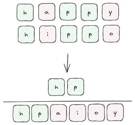
Like for $D_{\rm{hamming}}$, the Jaccard index is only concerned with the identity of the members in each set, so it can be applied to non-numerical members. In the case above, we see how the index can be calculated for the letters in two words.

You may have noted that the Jaccard index is a measure of similarity, rather than distance. It evaluates to 1 when the sets are identical and 0 when the sets have no overlap. To convert this index into a 'distance' measure we can just define $D_{\rm{jacccard}}$ to equal 1 minus the Jaccard index, i.e. $$ \begin{aligned} D_{\rm{jaccard}} \left( \mathbf{a}, \mathbf{b} \right) = 1 - \frac{ \left| \mathbf{a} \cap \mathbf{b} \right| }{ \left| \mathbf{a} \cup \mathbf{b} \right| } \tag{8}\label{8} \end{aligned} $$

We can implement this measure in ruby as follows

    
  def self.jaccard_similarity(a, b)
    return unless a.any? && b.any?

    1 - (a & b).size / (a | b).size.to_f
  end
    
  

Here we make use of Ruby's array set operators: & for intersection and | for union. If you want to brush up on these operators in ruby you can take a looks at our earlier post on array set operations in Ruby.

Summary

Machine learing algorithms often need to calculate the distance between two vectors, e.g. to find nearest neighbours. In this artice we have introduced 7 different ways of describing the distance between two vectors, and in each case have demonstrated how each of these measures can be simply implemented in ruby.

In ruby we can simply represent these vectors using the Array class. In all cases, except for the Jaccard distance, the two arrays must be of equal length in order to meaningfully apply the measure. Typically the measure will only make sense when dealing with numerical valued arrays, with the Hamming distance and Jaccard distance being exceptions to this. All other measures require two equal-length, numercial-valued arrays, and each measure is an extension of some concept of distance (or direction) familiar from 2D and 3D geometry.

I hope you found this article useful. If you have any feedback, questions or corrections please leave a comment below!

If you would like to be kept up-to-date when we publish new articles please subscribe.

References

1. 9 Distance Measures in Data Science, published on towardsdatascience.com
2. 7 Important Distance Metrics every Data Scientist should know, published on medium.com
3. Blog explaining the bag-of-words model for textual data
4. Simple GitHub repo with the metric implementations discussed in this post